Pulling Census Data with R
Have you ever wanted to access US census data so you could run your own analysis on them, rather than relying on the much more qualified data journalists and researchers to tell you what is in there? Me too! So I wrote a script to do just that. Check it out on Github if you want to follow along. You will need to request an API key from the US Census Bureau and save it in APIkey.txt for this script to work. The script that is shown below is the PopulationGraph.R file.
This post will run through this simple script that will pull age data from the American Community Survey 5 year data and plot it on a couple of line graphs.
Full disclosure, when I was googling around on how to do this, I mostly used this post from the University of Virginia libary to get it up and running. From there I updated the functions outlined for my own purposes. Alright, let’s jump in!
Library and Source Declarations
We start with the boring stuff. This first section declares all of our libraries and also loads in the API key.
rm(list=ls())
library (RJSONIO)
library(dplyr)
library(ggplot2)
library(tidyr)
source("ACSReqs.R")

# Import APIkey from text file.
fileName <- "APIkey.txt"
APIkey = readChar(fileName, file.info(fileName)$size)
Variable Definitions
Here we define out inputs to the census function. Since I am currently living in Tennessee, let’s start with that for our state. We will use every year available in the ACS 5 year data to get a larger dataset. We then assign the list of all Census data variables we want. Here we are pulling all of the simple “SEX by AGE” variables for the TN population. More details about these variables can be found in the ACS 5 year documentation here. We format these variables as a string separated by commas, as this is how the Census API will read them.
# Sate number for TN
state <- "47"
year <- c("2009","2010","2011","2012","2013","2014","2015","2016")

# Add all age variables by variable gender to the
varname <- paste("B01001_001E","B01001_002E","B01001_003E",
                 "B01001_004E","B01001_005E","B01001_006E",
                 "B01001_007E","B01001_008E","B01001_009E",
                 "B01001_010E","B01001_011E","B01001_012E",
                 "B01001_013E","B01001_014E","B01001_015E",
                 "B01001_016E","B01001_017E","B01001_018E",
                 "B01001_019E","B01001_020E","B01001_021E",
                 "B01001_022E","B01001_023E","B01001_024E",
                 "B01001_025E","B01001_026E","B01001_027E",
                 "B01001_028E","B01001_029E","B01001_030E",
                 "B01001_031E","B01001_032E","B01001_033E",
                 "B01001_034E","B01001_035E","B01001_036E",
                 "B01001_037E","B01001_038E","B01001_039E",
                 "B01001_040E","B01001_041E","B01001_042E",
                 "B01001_043E","B01001_044E","B01001_045E",
                 "B01001_046E","B01001_047E","B01001_048E",
                 "B01001_049E",sep=",")
Function Call and Definition
We are getting to the good stuff. Here we will loop over the year array that we created above and store it all in the ACS data Data Frame.
# Empty dataframe for combining all the data
ACSData <- data.frame()

# Actually pull all of the data from the API and combine it
for (i in year){
  print(i)
  temp <- getACSDataState("5",i,varname,state,APIkey)
  temp <- mutate(temp,Year=as.numeric(i))
  ACSData <- dplyr::bind_rows(ACSData,temp)
}
Pretty straightforward, but what is the getACSDataState function actually doing? It is defined in the ACSReqs.R file that we sourced at the top of the script and is shown below. The fucntion builds a request for the census api, submits it and pulls the results out using the fromJSON function. The results are converted into a dataframe (for now everything but the state number, and state name are changed to numeric).
getACSDataState <- function(ACSYear,year,varname,state,APIkey){
  # This function pulls data from the ACS API. Disclaimer: I have only tested 5 year data.
  #
  # Args:
  #   ACSYear: determine if accessing 1, 3, or 5 year data.
  #   year: Date of Census data
  #   varname: String of Census variables. They should be comma separated with no spaces.
  #   state: String representing the desired state. i.e. "47" for TN
  #   APIkey: API key requested from the US Census Bureau

  if(year=="2016" | year=="2015" | year=="2011"){
    resURL <- paste("http://api.census.gov/data/",year,"/acs/acs",ACSYear,"?get=NAME,",varname,
                  "&for=state:",state,"&key=",APIkey,sep="")
  }
  else{
    resURL <- paste("http://api.census.gov/data/",year,"/acs",ACSYear,"?get=NAME,",varname,
                    "&for=state:",state,"&key=",APIkey,sep="")
  }
  lJSON <- fromJSON(resURL)
  s <- gsub(",","",varname)
  count <- nchar(varname) - nchar(s) + 4
  lJSON.st <- sapply(lJSON, function(x) x[count-1])
  df <- data.frame(lJSON.st)
  for (i in 1:(count-2)){
    lJSON.temp <- sapply(lJSON, function(x) x[i])
    tempdf <- data.frame(lJSON.temp)
    df <- bind_cols(df, tempdf)
    next
  }
  colnames(df) <- as.character(unlist(df[1,]))
  df = df[-1,]
  ix <- 4:count-1
  df[ix] <- lapply(df[ix], as.character)
  df[ix] <- lapply(df[ix], as.numeric)
  return(df)
}
Manipulating the Data
Now that we have the data in the Data Frame, we will calculate the subsets we want by combining the totals from these variables and calculating the percentage of the population each group makes up using the total population B1001_003E value. Let’s split this data out into the classic marketing age groups: 18-24, 25-34, 35-44, 45-54, 55-65, and over 65. We will also include under 18, so no one is left out.
# Adding variables for Population percentage calculation
ACSData <- mutate(ACSData,
                  MalesUnder18=(B01001_003E+B01001_004E+B01001_005E+B01001_006E)/B01001_001E*100,
                  Males18to24=(B01001_007E+B01001_008E+B01001_009E+B01001_010E)/B01001_001E*100,
                  Males25to34=(B01001_011E+B01001_012E)/B01001_001E*100,
                  Males35to44=(B01001_013E+B01001_014E)/B01001_001E*100,
                  Males45to54=(B01001_015E+B01001_016E)/B01001_001E*100,
                  Males55to64=(B01001_017E+B01001_018E+B01001_019E)/B01001_001E*100,
                  MalesOver64=(B01001_020E+B01001_021E+B01001_022E+B01001_023E+B01001_024E+B01001_025E)/B01001_001E*100,
                  FemalesUnder18=(B01001_027E+B01001_028E+B01001_029E+B01001_030E)/B01001_001E*100,
                  Females18to24=(B01001_031E+B01001_032E+B01001_033E+B01001_034E)/B01001_001E*100,
                  Females25to34=(B01001_035E+B01001_036E)/B01001_001E*100,
                  Females35to44=(B01001_037E+B01001_038E)/B01001_001E*100,
                  Females45to54=(B01001_039E+B01001_040E)/B01001_001E*100,
                  Females55to64=(B01001_041E+B01001_042E+B01001_043E)/B01001_001E*100,
                  FemalesOver64=(B01001_044E+B01001_045E+B01001_046E+B01001_047E+B01001_048E+B01001_049E)/B01001_001E*100)
Plotting the Results
Now that we have calucalated our groups, let’s convert the data to a plottable format and give it a look.
# Select percent variables and convert from Wide to Tall for plotting
plotData <- ACSData[52:66]
tallData <- gather(plotData,"Group","Percent",2:15)
ggplot(data=tallData, aes(x=Year, y=Percent, group=Group)) +
       geom_line(aes(color=Group)) + geom_point(aes(color=Group)) +
       ggtitle("TN Population based on ACS Data - Gender")
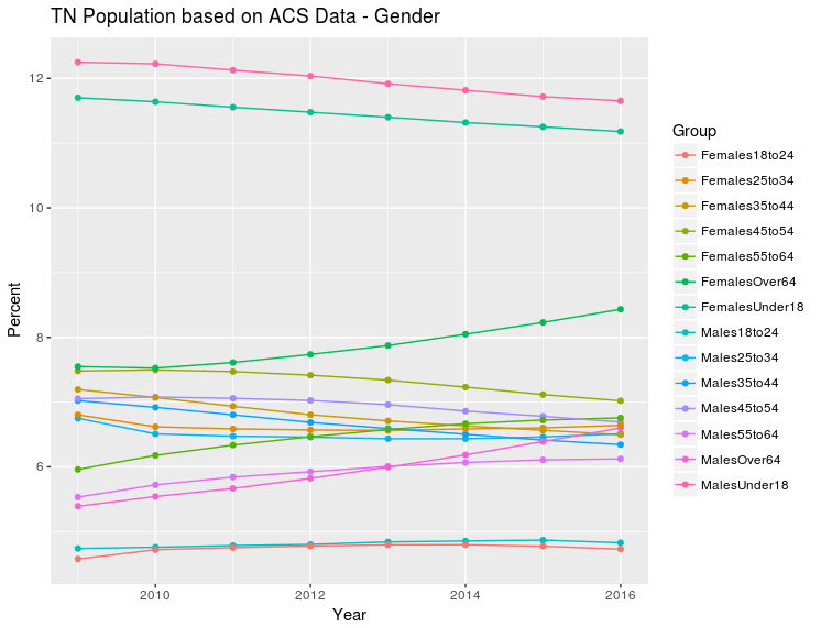
The code above gives us this graph:

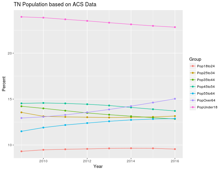
Hmmm, it is kind of hard to see any trends with such a busy graph. To fix this, we will combine the age groups and plot them again:
# Combine Gender percentages in ageData dataframe for plotting
ageData <- transmute(plotData, Year=Year,
                     PopUnder18=MalesUnder18+FemalesUnder18,
                     Pop18to24=Males18to24+Females18to24,
                     Pop25to34=Males25to34+Females25to34,
                     Pop35to44=Males35to44+Females35to44,
                     Pop45to54=Males45to54+Females45to54,
                     Pop55to64=Males55to64+Females55to64,
                     PopOver64=MalesOver64+FemalesOver64)
# Repeat plotting.
tallData2 <- gather(ageData,"Group","Percent",2:8)
ggplot(data=tallData2, aes(x=Year, y=Percent, group=Group)) +
       geom_line(aes(color=Group)) + geom_point(aes(color=Group)) +
       ggtitle("TN Population based on ACS Data")
Now that is much easier to see. And that wraps up the basics of accessing Census data and outputting it as a simple graph.
